Theory Hyperplane: w T x + b = 0 w^Tx+b=0 w T x + b = 0
w w w b: Intercept
x: Sample Points
y = +1 : Positive sample; y = -1: Negative Sample
Functional Margin γ i ^ = y i ( w T x i + b ) \hat{\gamma^{i}} = y^i(w^Tx^i+b) γ i ^ = y i ( w T x i + b )
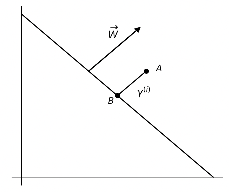
Geometric Margin The actual distance from the sample point to the hyperplane
x i x^i x i γ i {\gamma}^i γ i B A → \overrightarrow{BA} B A B: x i − γ i ⋅ W ∣ ∣ W ∣ ∣ x^i-{\gamma}_i \cdot \frac{W}{||W||} x i − γ i ⋅ ∣ ∣ W ∣ ∣ W
For B is on the line
w T ( x i − γ i ⋅ W ∣ ∣ W ∣ ∣ + b = 0 ) w^T(x^i-{\gamma}_i \cdot \frac{W}{||W||}+b=0) w T ( x i − γ i ⋅ ∣ ∣ W ∣ ∣ W + b = 0 ) Hence when y A = 1 y_A=1 y A = 1
γ i = w T x i + b ∣ ∣ w ∣ ∣ = ( w ∣ ∣ w ∣ ∣ ) T x i + b ∣ ∣ w ∣ ∣ {\gamma}^i=\frac{w^Tx^i+b}{||w||}={(\frac{w}{||w||})}^{T}x^i+\frac{b}{||w||} γ i = ∣ ∣ w ∣ ∣ w T x i + b = ( ∣ ∣ w ∣ ∣ w ) T x i + ∣ ∣ w ∣ ∣ b
More Generally
γ i = y i ( ( w ∣ ∣ w ∣ ∣ ) T x i + b ∣ ∣ w ∣ ∣ ) {\gamma}^i=y^i({(\frac{w}{||w||})}^{T}x^i+\frac{b}{||w||}) γ i = y i ( ( ∣ ∣ w ∣ ∣ w ) T x i + ∣ ∣ w ∣ ∣ b )
The functional margin is related to the geometric margin
γ = γ ^ ∣ ∣ w ∣ ∣ \gamma=\frac{\hat{\gamma}}{||w||} γ = ∣ ∣ w ∣ ∣ γ ^
Kernels Instead of utilizing SVMs with the original input attributes x, we might opt to train with certain features φ(x).ϕ ( x ) \phi(x) ϕ ( x ) ⟨ x , z ⟩ ⟨x,z⟩ ⟨ x , z ⟩ ⟨ ϕ ( x ) , ϕ ( z ) ⟩ ⟨\phi(x),\phi(z)⟩ ⟨ ϕ ( x ) , ϕ ( z ) ⟩
K ( x , z ) = ϕ ( x ) T ϕ ( z ) . K(x, z) = \phi(x)^{T}\phi(z). K ( x , z ) = ϕ ( x ) T ϕ ( z ) .
At every instance where we had ⟨x, z⟩ in our algorithm previously, Now, let’s talk about a slightly different view of kernels.K ( x , z ) = ϕ ( x ) T ϕ ( z ) K(x,z) = \phi(x)^{T}\phi(z) K ( x , z ) = ϕ ( x ) T ϕ ( z ) K ( x , z ) = ϕ ( x ) T ϕ ( z ) K(x, z) = \phi(x)^{T}\phi(z) K ( x , z ) = ϕ ( x ) T ϕ ( z )
K ( x , z ) = e x p ( − ∣ ∣ x − z ∣ ∣ 2 2 σ 2 ) = e x p ( − ∣ ∣ x ∣ ∣ 2 2 σ 2 ) e x p ( − ∣ ∣ z ∣ ∣ 2 2 σ 2 ) e x p ( ⟨ x , z ⟩ σ 2 ) K(x,z)=exp(\frac{-||x-z||^2}{2\sigma^2})=exp(\frac{-||x||^2}{2\sigma^2})exp(\frac{-||z||^2}{2\sigma^2})exp(\frac{\left\langle x, z\right\rangle}{\sigma^2}) K ( x , z ) = e x p ( 2 σ 2 − ∣ ∣ x − z ∣ ∣ 2 ) = e x p ( 2 σ 2 − ∣ ∣ x ∣ ∣ 2 ) e x p ( 2 σ 2 − ∣ ∣ z ∣ ∣ 2 ) e x p ( σ 2 ⟨ x , z ⟩ )
where the Taylor expansion for the third term is
e x p ( ⟨ x , z ⟩ σ 2 ) = 1 + ⟨ x , z ⟩ σ 2 + ⟨ x , z ⟩ 2 2 σ 4 + ⟨ x , z ⟩ 3 3 ! σ 6 + ⋯ = ∑ i = 0 n ⟨ x , z ⟩ n n ! ( σ ) n exp(\frac{ \left\langle x, z \right\rangle}{\sigma^2})=1+\frac{\left\langle x,z\right\rangle}{\sigma^2}+\frac{\left\langle x,z\right\rangle^2}{2\sigma^4}+\frac{\left\langle x,z\right\rangle^3}{3!\sigma^6}+\cdots=\sum\limits_{i=0}^n\frac{\left\langle x,z\right\rangle^n}{n!(\sigma)^n} e x p ( σ 2 ⟨ x , z ⟩ ) = 1 + σ 2 ⟨ x , z ⟩ + 2 σ 4 ⟨ x , z ⟩ 2 + 3 ! σ 6 ⟨ x , z ⟩ 3 + ⋯ = i = 0 ∑ n n ! ( σ ) n ⟨ x , z ⟩ n
Due to the existence of the Taylor expansion, the mapping from low to infinite dimensions is achieved with the help of the Gaussian Kernel or Radial Basis Function (RBF)
Common Kernel Functions Linear Kernel K ( x , z ) = ⟨ x , z ⟩ K(x,z)=\left\langle x,z \right\rangle K ( x , z ) = ⟨ x , z ⟩
Polynomial Kernel K ( x , z ) = ( γ ⟨ x , z ⟩ + r ) d K(x,z)=(\gamma\left\langle x,z \right\rangle + r)^d K ( x , z ) = ( γ ⟨ x , z ⟩ + r ) d
Gaussian Kernel K ( x , z ) = e x p ( − γ ∣ ∣ x − z ∣ ∣ 2 ) K(x,z)=exp(-\gamma||x-z||^2) K ( x , z ) = e x p ( − γ ∣ ∣ x − z ∣ ∣ 2 )
Sigmoid Kernel K ( x , z ) = t a n h ( γ ⟨ x , z ⟩ + r ) K(x,z)=tanh(\gamma\left\langle x,z \right\rangle + r) K ( x , z ) = t a n h ( γ ⟨ x , z ⟩ + r )
Lagrange Multipliers In mathematical optimization, the method of Lagrange multipliers is a strategy for finding the local maxima and minima of a function subject to equality constraintsz = f ( x , y , z , ⋯ ) z = f(x,y,z,\cdots) z = f ( x , y , z , ⋯ ) ϕ ( x , y , … ) = 0 , ψ ( x , y , … ) = 0 \phi(x,y,\ldots) = 0, \quad \psi(x,y,\ldots) = 0 ϕ ( x , y , … ) = 0 , ψ ( x , y , … ) = 0
Make a Lagrangian function
F ( x , y , z , ⋯ , λ , ν , ⋯ ) = f ( x , y , z , ⋯ ) + μ ϕ ( x , y , ⋯ ) + μ ϕ ( x , y , ⋯ ) + μ ϕ ( x , y , ⋯ ) F(x,y,z,\cdots,\lambda,\nu,\cdots)=f(x,y,z,\cdots)+ \mu\phi(x,y,\cdots)+\mu\phi(x,y,\cdots)+\mu\phi(x,y,\cdots) F ( x , y , z , ⋯ , λ , ν , ⋯ ) = f ( x , y , z , ⋯ ) + μ ϕ ( x , y , ⋯ ) + μ ϕ ( x , y , ⋯ ) + μ ϕ ( x , y , ⋯ ) Find the stationary points of the multivariate function F ( x , t , z , ⋯ , λ , μ , ⋯ ) F(x,t,z,\cdots,\lambda,\mu,\cdots) F ( x , t , z , ⋯ , λ , μ , ⋯ ) ( x 0 , y 0 , z 0 , ⋯ , λ 0 , μ 0 , ⋯ ) (x_0,y_0,z_0,\cdots,\lambda_0,\mu_0,\cdots) ( x 0 , y 0 , z 0 , ⋯ , λ 0 , μ 0 , ⋯ )
then f ( x 0 , y 0 , z 0 , ⋯ ) f(x_0,y_0,z_0,\cdots) f ( x 0 , y 0 , z 0 , ⋯ )
{ F x = 0 F y = 0 ⋯ F λ = 0 ⋯
\left\{
\begin{array}{c}
F_x=0 \\
F_y=0 \\
\cdots \\
F_{\lambda}=0\\
\cdots
\end{array}
\right.
⎩ ⎪ ⎪ ⎪ ⎪ ⎪ ⎨ ⎪ ⎪ ⎪ ⎪ ⎪ ⎧ F x = 0 F y = 0 ⋯ F λ = 0 ⋯
Now f ( x 0 , y 0 , z 0 ) f(x_0,y_0,z_0) f ( x 0 , y 0 , z 0 ) Generalized Lagranigian L ( w , α , β ) = f ( w ) + ∑ i = 1 k α i g i ( w ) + ∑ i = 1 l β i h i ( w ) L(w,\alpha,\beta)=f(w)+\sum\limits_{i=1}^k\alpha_ig_i(w)+\sum\limits_{i=1}^l\beta_ih_i(w) L ( w , α , β ) = f ( w ) + i = 1 ∑ k α i g i ( w ) + i = 1 ∑ l β i h i ( w )
Here, the α i \alpha_i α i β i \beta_i β i θ P ( w ) = max α , β : α i ≥ 0 L ( w , α , β ) \theta_{P}(w)= \max \limits_{\alpha,\beta : \alpha_i \geq 0} L(w,\alpha,\beta) θ P ( w ) = α , β : α i ≥ 0 max L ( w , α , β )
P stands for “Primal”g i ( w ) ≤ 0 g_i(w) \leq 0 g i ( w ) ≤ 0 h i ( w ) = 0 h_i(w)=0 h i ( w ) = 0 w w w
θ p ( w ) = max α , β : α i ≥ 0 ( ∑ i = 1 k α i g i ( w ) + ∑ i = 1 l β i h i ( w ) ) \theta_p(w)=\max\limits_{\alpha,\beta:\alpha_i \geq 0}(\sum\limits_{i=1}^{k}\alpha_ig_i(w)+\sum\limits_{i=1}^{l}\beta_{i} h_i(w)) θ p ( w ) = α , β : α i ≥ 0 max ( i = 1 ∑ k α i g i ( w ) + i = 1 ∑ l β i h i ( w ) ) which means
θ p ( w ) = f ( w ) + 0 \theta_p(w)=f(w)+0 θ p ( w ) = f ( w ) + 0 If the constraints are not satisfied
θ p ( w ) = ∞ \theta_p(w)=\infty θ p ( w ) = ∞
Dual Optimization Problem Define
θ D ( α , β ) = min w L ( w , α , β ) \theta_D(\alpha,\beta)=\min\limits_{w}L(w,\alpha,\beta) θ D ( α , β ) = w min L ( w , α , β )
D stands for dual
We can now pose the dual optimization problem:
d ∗ = max α , β : α i ≥ 0 θ D ( α , β ) = max α , β : α i ≥ 0 min w L ( w , α , β ) d^{*}=\max\limits_{\alpha,\beta:\alpha_i \geq 0}\theta_{D}(\alpha,\beta)=\max\limits_{\alpha,\beta:\alpha_i \geq 0}\min\limits_{w}L(w,\alpha,\beta) d ∗ = α , β : α i ≥ 0 max θ D ( α , β ) = α , β : α i ≥ 0 max w min L ( w , α , β )
The primal and the dual problem are related like this:
d ∗ = max α , β : α i ≥ 0 L ( w , α , β ) ≤ min w max α , β : α i ≥ 0 L ( w , α , β ) = p ∗ d^{*}=\max\limits_{\alpha,\beta: \alpha_i \geq 0}L(w,\alpha,\beta) \leq \min\limits_{w} \max\limits_{\alpha,\beta:\alpha_i \geq 0}L(w,\alpha,\beta)=p^{*} d ∗ = α , β : α i ≥ 0 max L ( w , α , β ) ≤ w min α , β : α i ≥ 0 max L ( w , α , β ) = p ∗
Karush-Kuhn-Tucker(KKT) Suppose f ( w ) f(w) f ( w ) g i ( w ) g_i(w) g i ( w ) h i h_i h i g i g_i g i w w w g i ( w ) ≤ 0 g_i(w) \le 0 g i ( w ) ≤ 0 i i i w ∗ , α ∗ , β ∗ w_*, \alpha_*, \beta_* w ∗ , α ∗ , β ∗ w ∗ w_* w ∗ α ∗ , β ∗ \alpha_*,\beta_* α ∗ , β ∗ p ∗ = d ∗ = L ( w ∗ , α ∗ , β ∗ ) p_* = d_* = L(w_*, \alpha_*, \beta_*) p ∗ = d ∗ = L ( w ∗ , α ∗ , β ∗ )
w ∗ , α ∗ a n d β ∗ w_*, \alpha_* and \beta_* w ∗ , α ∗ a n d β ∗ ∂ ∂ w i L ( w ∗ , α ∗ , β ∗ ) = 0 , i = 1 , … , d ∂ ∂ β i L ( w ∗ , α ∗ , β ∗ ) = 0 , i = 1 , … , l α i ∗ g i ( w ∗ ) = 0 , i = 1 , … , k g i ( w ∗ ) ≤ 0 , i = 1 , … , k α ∗ ≥ 0 , i = 1 , … , k \begin{aligned} \frac{\partial}{\partial w_i} \mathcal{L}\left(w^*, \alpha^*, \beta^*\right) & =0, i=1, \ldots, d \\ \frac{\partial}{\partial \beta_i} \mathcal{L}\left(w^*, \alpha^*, \beta^*\right) & =0, i=1, \ldots, l \\ \alpha_i^* g_i\left(w^*\right) & =0, i=1, \ldots, k \\ g_i\left(w^*\right) & \leq 0, i=1, \ldots, k \\ \alpha^* & \geq 0, i=1, \ldots, k\end{aligned} ∂ w i ∂ L ( w ∗ , α ∗ , β ∗ ) ∂ β i ∂ L ( w ∗ , α ∗ , β ∗ ) α i ∗ g i ( w ∗ ) g i ( w ∗ ) α ∗ = 0 , i = 1 , … , d = 0 , i = 1 , … , l = 0 , i = 1 , … , k ≤ 0 , i = 1 , … , k ≥ 0 , i = 1 , … , k α i ∗ g i ( w ∗ ) = 0 \alpha_i^* g_i(w^*) =0 α i ∗ g i ( w ∗ ) = 0 Specifically, it implies that if α i ∗ ≥ 0 α_i^{*} \ge 0 α i ∗ ≥ 0 g i ( w ∗ ) = 0 g_i(w^*) = 0 g i ( w ∗ ) = 0
Optimization Hard Margin Find the local minimal value W(a) of L with w and b The final optimization objective of the SVM hard margin is
min w , b 1 2 ∣ ∣ w ∣ ∣ 2 \min\limits_{w,b}\frac{1}{2}||w||^2 w , b min 2 1 ∣ ∣ w ∣ ∣ 2
s . t . y ( i ) ( w T x ( i ) + b ) ≥ 1 , i = 1 , ⋯ , n s.t. y^{(i)}(w^Tx^{(i)}+b) \geq 1, i=1,\cdots,n s . t . y ( i ) ( w T x ( i ) + b ) ≥ 1 , i = 1 , ⋯ , n
The Generalized Lagranigian Function is:
L ( w , b , α ) = 1 2 ∣ ∣ w ∣ ∣ 2 − ∑ i = 1 m α i [ y ( i ) ( w T x ( i ) + b ) − 1 ] L(w,b,\alpha)=\frac{1}{2}||w||^2-\sum\limits_{i=1}^m\alpha_i[y^{(i)}(w^{T}x^{(i)}+b)-1] L ( w , b , α ) = 2 1 ∣ ∣ w ∣ ∣ 2 − i = 1 ∑ m α i [ y ( i ) ( w T x ( i ) + b ) − 1 ]
where \alpha_i≥0 is the Lagrangian multiplier
g i ( w ) = − y ( i ) ( w T x ( i ) + b ) + 1 ≤ 0 g_i(w)=-y^{(i)}(w^{T}x^{(i)}+b)+1 \leq 0 g i ( w ) = − y ( i ) ( w T x ( i ) + b ) + 1 ≤ 0
Then the original problem’s dual optimization problem is:
d ∗ = max α , α i ≥ 0 min w , b L ( w , b , α ) d^* = \max\limits_{\alpha,\alpha_i \geq 0}\min\limits_{w,b}L(w,b,\alpha) d ∗ = α , α i ≥ 0 max w , b min L ( w , b , α )
To solve this,we need to calculate the partial derivatives for w and b and make it to zero.
∂ L ∂ w = w − ∑ i = 1 m α i y ( i ) x ( i ) = 0 \frac{\partial L}{\partial w}=w-\sum\limits_{i=1}^m \alpha_{i}y^{(i)}x^{(i)}=0 ∂ w ∂ L = w − i = 1 ∑ m α i y ( i ) x ( i ) = 0
∂ L ∂ b = − ∑ i = 1 m α i y ( i ) = 0 \frac{\partial L}{\partial b}=-\sum\limits_{i=1}^m\alpha_{i}y^{(i)}=0 ∂ b ∂ L = − i = 1 ∑ m α i y ( i ) = 0
Then we have
w = ∑ i = 1 m α i y ( i ) w=\sum\limits_{i=1}^m\alpha_i y^{(i)} w = i = 1 ∑ m α i y ( i )
W ( α ) = min w , b L ( w , b , α ) = ∑ i = 1 m α i − 1 2 ∑ i , j = 1 m y ( i ) y ( j ) α i α j ( x ( i ) ) T x ( j ) W(\alpha)=\min\limits_{w,b}L(w,b,\alpha)=\sum\limits_{i=1}^{m}\alpha_i-\frac{1}{2}\sum\limits_{i,j=1}^{m}y_{(i)}y_{(j)}\alpha_i\alpha_j(x^{(i)})^{T}x^{(j)} W ( α ) = w , b min L ( w , b , α ) = i = 1 ∑ m α i − 2 1 i , j = 1 ∑ m y ( i ) y ( j ) α i α j ( x ( i ) ) T x ( j )
Solution Steps:
L ( w , b , a ) = 1 2 w T w − ∑ i = 1 m α , [ y ( 1 ) ( w T x ( i ) + b ) − 1 ] = 1 2 w T w − ∑ i = 1 m α i y ( i ) w T x ( i ) − ∑ i = 1 m α i y ( i ) b + ∑ i = 1 ∞ α i = 1 2 w T w − w T ∑ i = 1 m α i y ( i ) x ( i ) − b ∑ i = 1 m a i y ( i ) + ∑ i = 1 m α i \begin{aligned}
L(w, b, a)&=\frac{1}{2} w^{T} w-\sum_{i=1}^m \alpha,\left[y^{(1)}\left(w^{T} x^{(i)}+b\right)-1\right] \\
& =\frac{1}{2} w^{\mathrm{T}} w-\sum_{i=1}^m \alpha_i y^{(i)} w^{\mathrm{T}} x^{(i)}-\sum_{i=1}^m \alpha_i y^{(i)} b+\sum_{i=1}^{\infty} \alpha_i \\
& =\frac{1}{2} w^{T} w-w^{T} \sum_{i=1}^m \alpha_i y^{(i)} x^{(i)}-b \sum_{i=1}^m a_i y^{(i)}+\sum_{i=1}^m \alpha_i \\
&
\end{aligned}
L ( w , b , a ) = 2 1 w T w − i = 1 ∑ m α , [ y ( 1 ) ( w T x ( i ) + b ) − 1 ] = 2 1 w T w − i = 1 ∑ m α i y ( i ) w T x ( i ) − i = 1 ∑ m α i y ( i ) b + i = 1 ∑ ∞ α i = 2 1 w T w − w T i = 1 ∑ m α i y ( i ) x ( i ) − b i = 1 ∑ m a i y ( i ) + i = 1 ∑ m α i
W ( α ) = 1 2 w T w − w T w + ∑ i = 1 m α i = ∑ i = 1 m α i − 1 2 w ⊤ w = ∑ i = 1 m α i − 1 2 ∑ i , j = 1 m α i α i y ( i ) y ( j ) ( x ( i ) ) T x ( j )
\begin{aligned}
W(\alpha) & =\frac{1}{2} w^{T} w-w^{T} w+\sum_{i=1}^m \alpha_i \\
& =\sum_{i=1}^m \alpha_i-\frac{1}{2} w^{\top} w \\
& =\sum_{i=1}^m \alpha_i-\frac{1}{2} \sum_{i, j=1}^m \alpha_i \alpha_i y^{(i)} y^{(j)}\left(x^{(i)}\right)^T x^{(j)}
\end{aligned}
W ( α ) = 2 1 w T w − w T w + i = 1 ∑ m α i = i = 1 ∑ m α i − 2 1 w ⊤ w = i = 1 ∑ m α i − 2 1 i , j = 1 ∑ m α i α i y ( i ) y ( j ) ( x ( i ) ) T x ( j ) Hence
W ( α ) = min w , b L ( w , b , α ) = ∑ i = 1 n α i − 1 2 ∑ i , j = 1 n y ( i ) y ( j ) α i α j ( x ( i ) ) T x ( j ) W(\alpha)=\min\limits_{w, b}\mathcal{L}(w, b, \alpha)=\sum\limits_{i=1}^n \alpha_i-\frac{1}{2} \sum\limits_{i, j=1}^n y^{(i)} y^{(j)} \alpha_i \alpha_j\left(x^{(i)}\right)^T x^{(j)} W ( α ) = w , b min L ( w , b , α ) = i = 1 ∑ n α i − 2 1 i , j = 1 ∑ n y ( i ) y ( j ) α i α j ( x ( i ) ) T x ( j )
Find the local maximum value W(a) of L with a Consider an optimization Problem:
max W ( α ) = max ∑ i = 1 m α 1 − 1 2 ∑ i , j = 1 m y ( i ) y ( j ) α i α j ( x ( i ) ) ⊤ x ( 0 ) s. t. α i ⩾ 0 , i = 1 , 2 , ⋯ , m \begin{aligned} & \max W(\alpha)=\max \sum_{i=1}^m \alpha_1-\frac{1}{2} \sum\limits_{i,j=1}^{m} y^{(i)} y^{(j)} \alpha_i \alpha_j\left(x^{(i)}\right)^{\top} x^{(0)} \\ & \text { s. t. } \alpha_i \geqslant 0, \quad i=1,2, \cdots, m\end{aligned} max W ( α ) = max i = 1 ∑ m α 1 − 2 1 i , j = 1 ∑ m y ( i ) y ( j ) α i α j ( x ( i ) ) ⊤ x ( 0 ) s. t. α i ⩾ 0 , i = 1 , 2 , ⋯ , m
With the constraint Condition:
∑ i = 1 m α i y ( i ) = 0 \sum\limits_{i=1}^{m} \alpha_{i} y^{(i)}=0 i = 1 ∑ m α i y ( i ) = 0
Furthermore,suppose α ∗ = ( α 1 ∗ , α 2 ∗ , ⋯ , α m ∗ ) T \alpha^*=(\alpha_1^*,\alpha_2^*,\cdots, \alpha_m^*)^T α ∗ = ( α 1 ∗ , α 2 ∗ , ⋯ , α m ∗ ) T
∂ ∂ w L ( w ∗ , b ∗ , α ∗ ) = w ∗ − ∑ i = 1 m α i ∗ y ( i ) x ( i ) = 0 ∂ ∂ b L ( w ∗ , b ∗ , α ∗ ) = − ∑ i = 1 m α i ∗ y ( i ) = 0 α i ∗ g i ( w ∗ ) = α i ∗ [ y ( i ) ( w ∗ ⋅ x ( i ) + b ∗ ) − 1 ] = 0 , i = 1 , 2 , ⋯ , m g i ( w ∗ ) = − y ( i ) ( w ∗ ⋅ x ( i ) + b ∗ ) + 1 ⩽ 0 , i = 1 , 2 , ⋯ , m α i ∗ ⩾ 0 , i = 1 , 2 , ⋯ , m \begin{aligned} & \frac{\partial}{\partial w} L\left(w^*, b^*, \alpha^*\right)=w^*-\sum_{i=1}^m \alpha_i^* y^{(i)} x^{(i)}=0 \\ & \frac{\partial}{\partial b} L\left(w^*, b^*, \alpha^*\right)=-\sum_{i=1}^m \alpha_i^* y^{(i)}=0 \\ & \alpha_i^* g_i\left(w^*\right)=\alpha_i^*\left[y^{(i)}\left(w^* \cdot x^{(i)}+b^*\right)-1\right]=0, \quad i=1,2, \cdots, m \\ & g_i\left(w^*\right)=-y^{(i)}\left(w^* \cdot x^{(i)}+b^*\right)+1 \leqslant 0, \quad i=1,2, \cdots, m \\
& \alpha_i^* \geqslant 0, \quad i=1,2, \cdots, m \end{aligned} ∂ w ∂ L ( w ∗ , b ∗ , α ∗ ) = w ∗ − i = 1 ∑ m α i ∗ y ( i ) x ( i ) = 0 ∂ b ∂ L ( w ∗ , b ∗ , α ∗ ) = − i = 1 ∑ m α i ∗ y ( i ) = 0 α i ∗ g i ( w ∗ ) = α i ∗ [ y ( i ) ( w ∗ ⋅ x ( i ) + b ∗ ) − 1 ] = 0 , i = 1 , 2 , ⋯ , m g i ( w ∗ ) = − y ( i ) ( w ∗ ⋅ x ( i ) + b ∗ ) + 1 ⩽ 0 , i = 1 , 2 , ⋯ , m α i ∗ ⩾ 0 , i = 1 , 2 , ⋯ , m w ∗ = ∑ i = 1 m α i ∗ y ( i ) x ( i ) w^*=\sum\limits_{i=1}^m\alpha_i^*y^{(i)}x^{(i)} w ∗ = i = 1 ∑ m α i ∗ y ( i ) x ( i )
So at least there exists one α j ≥ 0 ∗ \alpha_j^ \ge 0{*} α j ≥ 0 ∗ if α j ≥ 0 ∗ \alpha_j^ \ge 0{*} α j ≥ 0 ∗
y ( j ) ( w ∗ ⋅ x ( j ) + b ∗ ) = 1 y^{(j)}(w^* \cdot x^{(j)}+b^*)=1 y ( j ) ( w ∗ ⋅ x ( j ) + b ∗ ) = 1
From this we got that the sample point x ( j ) x^{(j)} x ( j ) Moreover,for ( y ( j ) = 1 ) (y^{(j)}=1) ( y ( j ) = 1 )
b ∗ = y ( j ) − ∑ i = 1 m α i ∗ y ( i ) ( x ( i ) ⋅ x ( j ) ) b^* = y^{(j)}-\sum\limits_{i=1}^m\alpha_{i}^*y^{(i)}(x^(i) \cdot x^(j)) b ∗ = y ( j ) − i = 1 ∑ m α i ∗ y ( i ) ( x ( i ) ⋅ x ( j ) )
Soft Margin The final optimization objective of the SVM hard margin is
min w , b 1 2 ∣ ∣ w ∣ ∣ 2 + C ∑ i = 1 m ζ i \min\limits_{w,b}\frac{1}{2}||w||^2 + C\sum\limits_{i=1}^{m} \zeta_i w , b min 2 1 ∣ ∣ w ∣ ∣ 2 + C i = 1 ∑ m ζ i
s . t . y ( i ) ( w T x ( i ) + b ) ≥ 1 − ζ i , ζ i ≥ 0 , i = 1 , 2 , ⋯ , m s.t. y^{(i)}(w^Tx^{(i)}+b)\geq 1- \zeta_i,\zeta_i \geq 0, i=1,2,\cdots,m s . t . y ( i ) ( w T x ( i ) + b ) ≥ 1 − ζ i , ζ i ≥ 0 , i = 1 , 2 , ⋯ , m
Then the generalized lagranigian function is:
L ( w , b , ζ , α , r ) = 1 2 ∥ w ∥ 2 + C ∑ i = 1 m ζ i − ∑ i = 1 m α i [ y ( i ) ( w T x ( i ) + b ) − 1 + ζ i ] − ∑ i = 1 m r i ζ i L(w, b, \zeta, \alpha, r)=\frac{1}{2}\|w\|^2+C \sum_{i=1}^m \zeta_i-\sum_{i=1}^m \alpha_i\left[y^{(i)}\left(w^{T} x^{(i)}+b\right)-1+\zeta_i\right]-\sum_{i=1}^m r_i \zeta_i L ( w , b , ζ , α , r ) = 2 1 ∥ w ∥ 2 + C ∑ i = 1 m ζ i − ∑ i = 1 m α i [ y ( i ) ( w T x ( i ) + b ) − 1 + ζ i ] − ∑ i = 1 m r i ζ i
Among which α i ≥ 0 \alpha_i \geq 0 α i ≥ 0 r i ≥ 0 r_i \geq 0 r i ≥ 0
{ g i ( w ) = − y ( i ) ( w T x ( i ) + b ) + 1 − ζ i ⩽ 0 h i ( ζ ) = − ζ i ⩽ 0 ; i = 1 , 2 , ⋯ , m \left\{\begin{array}{l}g_i(w)=-y^{(i)}\left(w^{T} x^{(i)}+b\right)+1-\zeta_i \leqslant 0 \\ h_i(\zeta)=-\zeta_i \leqslant 0 ; \quad i=1,2, \cdots, m\end{array}\right. { g i ( w ) = − y ( i ) ( w T x ( i ) + b ) + 1 − ζ i ⩽ 0 h i ( ζ ) = − ζ i ⩽ 0 ; i = 1 , 2 , ⋯ , m
So we can get the dual optimization problem of the primal optimization problem
d ∗ = max α , r min w , b , ζ L ( w , b , ζ , α , r ) d^*=\max\limits_{\alpha,r}\min\limits_{w,b,\zeta}L(w,b,\zeta,\alpha,r) d ∗ = α , r max w , b , ζ min L ( w , b , ζ , α , r )
Find the local minimal value W(a,r) of L with w ,b and ζ \zeta ζ ∂ L ∂ w = w − ∑ i = 1 m α i y ( i ) x ( i ) = 0 \frac{\partial L}{\partial w}=w-\sum\limits_{i=1}^{m}\alpha_{i}y^{(i)}x^{(i)}=0 ∂ w ∂ L = w − i = 1 ∑ m α i y ( i ) x ( i ) = 0
∂ L ∂ b = − ∑ i = 1 m α i y ( i ) = 0 ∂ L ∂ ζ i = C − α i − r i = 0 w = ∑ i = 1 m α i y ( i ) x ( i ) ∑ i = 1 m α i y ( i ) = 0 C − α i − r i = 0 \begin{gathered}\frac{\partial L}{\partial b}=-\sum_{i=1}^m \alpha_i y^{(i)}=0 \\ \frac{\partial L}{\partial \zeta_i}=C-\alpha_i-r_i=0 \\ w=\sum_{i=1}^m \alpha_i y^{(i)} x^{(i)} \\ \sum_{i=1}^m \alpha_i y^{(i)}=0 \\ C-\alpha_i-r_i=0\end{gathered} ∂ b ∂ L = − i = 1 ∑ m α i y ( i ) = 0 ∂ ζ i ∂ L = C − α i − r i = 0 w = i = 1 ∑ m α i y ( i ) x ( i ) i = 1 ∑ m α i y ( i ) = 0 C − α i − r i = 0
Further
W ( α , r ) = 1 2 w T w + C ∑ i = 1 m ζ i − w T w + ∑ i = 1 m α i − ∑ i = 1 m α i ζ i − ∑ i = 1 m r i ζ i = ∑ i = 1 m α i − 1 2 w T w + ∑ i = 1 m ζ i ( C − α i − r i ) = ∑ i = 1 m α i − 1 2 w T w \begin{aligned}
W(\alpha, r) & =\frac{1}{2} w^{\mathrm{T}} w+C \sum_{i=1}^m \zeta_i-w^{\mathrm{T}} w+\sum_{i=1}^m \alpha_i-\sum_{i=1}^m \alpha_i \zeta_i-\sum_{i=1}^m r_i \zeta_i \\
& =\sum_{i=1}^m \alpha_i-\frac{1}{2} w^{\mathrm{T}} w+\sum_{i=1}^m \zeta_i\left(C-\alpha_i-r_i\right) \\
& =\sum_{i=1}^m \alpha_i-\frac{1}{2} w^{\mathrm{T}} w
\end{aligned} W ( α , r ) = 2 1 w T w + C i = 1 ∑ m ζ i − w T w + i = 1 ∑ m α i − i = 1 ∑ m α i ζ i − i = 1 ∑ m r i ζ i = i = 1 ∑ m α i − 2 1 w T w + i = 1 ∑ m ζ i ( C − α i − r i ) = i = 1 ∑ m α i − 2 1 w T w
Find the local maximum value W(a) of L with α \alpha α From the following calculation to find the local maximum of \alpha we have:
max a W ( α ) = max a ∑ i = 1 m α i − 1 2 w T w s. t. ∑ i = 1 m α i y ( i ) = 0 C − α i − r i = 0 , i = 1 , 2 , ⋯ , m α i ⩾ 0 , i = 1 , 2 , ⋯ , m r i ⩾ 0 , i = 1 , 2 , ⋯ , m \begin{aligned}
& \max _a W(\alpha)=\max _a \sum_{i=1}^m \alpha_i-\frac{1}{2} w^{\mathrm{T}} w \\
& \text { s. t. } \sum_{i=1}^m \alpha_i y^{(i)}=0 \\
& C-\alpha_i-r_i=0, \quad i=1,2, \cdots, m \\
& \alpha_i \geqslant 0, \quad i=1,2, \cdots, m \\
& r_i \geqslant 0, \quad i=1,2, \cdots, m
\end{aligned} a max W ( α ) = a max i = 1 ∑ m α i − 2 1 w T w s. t. i = 1 ∑ m α i y ( i ) = 0 C − α i − r i = 0 , i = 1 , 2 , ⋯ , m α i ⩾ 0 , i = 1 , 2 , ⋯ , m r i ⩾ 0 , i = 1 , 2 , ⋯ , m Then we can get the constraint condition:
0 ≤ α i ≤ C 0 \leq \alpha_i \leq C 0 ≤ α i ≤ C Finally, we can get the final dual optimization problem:
max α ∑ i = 1 m α i − 1 2 ∑ i , j = 1 m y ( i ) y ( j ) α i α j ( x ( i ) ) T x ( j ) s. t. 0 ⩽ α i ⩽ C , i = 1 , 2 , ⋯ , m and ∑ i = 1 m α i y ( i ) = 0 \begin{aligned}
& \max _\alpha \sum_{i=1}^m \alpha_i-\frac{1}{2} \sum_{i, j=1}^m y^{(i)} y^{(j)} \alpha_i \alpha_j\left(x^{(i)}\right)^{\mathrm{T}} x^{(j)} \\
& \text { s. t. } 0 \leqslant \alpha_i \leqslant C, \quad i=1,2, \cdots, m \quad \text { and } \quad \sum_{i=1}^m \alpha_i y^{(i)}=0
\end{aligned} α max i = 1 ∑ m α i − 2 1 i , j = 1 ∑ m y ( i ) y ( j ) α i α j ( x ( i ) ) T x ( j ) s. t. 0 ⩽ α i ⩽ C , i = 1 , 2 , ⋯ , m and i = 1 ∑ m α i y ( i ) = 0
Now suppose α ∗ = ( α 1 1 ∗ , α 2 ∗ , ⋯ , α m ∗ ) T \alpha^*=(\alpha_1^1*,\alpha_2^*,\cdots,\alpha_m^*)^T α ∗ = ( α 1 1 ∗ , α 2 ∗ , ⋯ , α m ∗ ) T
∂ ∂ w L ( w ∗ , b ∗ , ζ ∗ , α ∗ , r ∗ ) = w ∗ − ∑ i = 1 ∞ α i y ( i ) x ( i ) = 0 ∂ ∂ b L ( w ∗ , b ∗ , ζ ∗ , α ∗ , r ∗ ) = − ∑ i = 1 ∞ α i y ( i ) = 0 ∂ ∂ ζ L ( w ∗ , b ∗ , ζ ∗ ⋅ α ∗ , r ∗ ) = C − α ∗ − r ∗ = 0 α i ∗ g i ( w ∗ ) = α i ∗ [ y ( i ) ( w ∗ ⋅ x ( i ) + b ∗ ) − 1 + ζ i ] = 0 , i = 1 , 2 , ⋯ , m r i ∗ h i ( ζ ∗ ) = r i ∗ ζ i ∗ = 0 ; i = 1 , 2 , ⋯ , m g i ( w ∗ ) = − y ( i ) ( w ∗ ⋅ x ( i ) + b ∗ ) + 1 − ζ i ⩽ 0 , i = 1 , 2 , ⋯ , m h i ( ζ ∗ ) = − ζ i ⩽ 0 ; i = 1 , 2 , ⋯ , m α i ∗ ⩾ 0 , r i ∗ ⩾ 0 ; i = 1 , 2 , ⋯ , m \begin{aligned}
& \frac{\partial}{\partial w} L\left(w^*, b^*, \zeta^*, \alpha^*, r^*\right)=w^*-\sum\limits_{i=1}^{\infty} \alpha_i y^{(i)} x^{(i)}=0 \\
& \frac{\partial}{\partial b} L\left(w^*, b^*, \zeta^*, \alpha^*, r^*\right)=-\sum\limits_{i=1}^{\infty} \alpha_i y^{(i)}=0 \\
& \frac{\partial}{\partial \zeta} L\left(w^*, b^*, \zeta^* \cdot \alpha^*, r^*\right)=C-\alpha^*-r^*=0 \\
& \alpha_i^* g_i\left(w^*\right)=\alpha_i^*\left[y^{(i)}\left(w^* \cdot x^{(i)}+b^*\right)-1+\zeta_i\right]=0, \quad i=1,2, \cdots, m \\
& r_i^* h_i\left(\zeta^*\right)=r_i^* \zeta_i^*=0 ; \quad i=1,2, \cdots, m \\
& g_i\left(w^*\right)=-y^{(i)}\left(w^* \cdot x^{(i)}+b^*\right)+1-\zeta_i \leqslant 0, \quad i=1,2, \cdots, m \\
& h_i\left(\zeta^*\right)=-\zeta_i \leqslant 0 ; \quad i=1,2, \cdots, m \\
& \alpha_i^* \geqslant 0, \quad r_i^* \geqslant 0 ; \quad i=1,2, \cdots, m
\end{aligned} ∂ w ∂ L ( w ∗ , b ∗ , ζ ∗ , α ∗ , r ∗ ) = w ∗ − i = 1 ∑ ∞ α i y ( i ) x ( i ) = 0 ∂ b ∂ L ( w ∗ , b ∗ , ζ ∗ , α ∗ , r ∗ ) = − i = 1 ∑ ∞ α i y ( i ) = 0 ∂ ζ ∂ L ( w ∗ , b ∗ , ζ ∗ ⋅ α ∗ , r ∗ ) = C − α ∗ − r ∗ = 0 α i ∗ g i ( w ∗ ) = α i ∗ [ y ( i ) ( w ∗ ⋅ x ( i ) + b ∗ ) − 1 + ζ i ] = 0 , i = 1 , 2 , ⋯ , m r i ∗ h i ( ζ ∗ ) = r i ∗ ζ i ∗ = 0 ; i = 1 , 2 , ⋯ , m g i ( w ∗ ) = − y ( i ) ( w ∗ ⋅ x ( i ) + b ∗ ) + 1 − ζ i ⩽ 0 , i = 1 , 2 , ⋯ , m h i ( ζ ∗ ) = − ζ i ⩽ 0 ; i = 1 , 2 , ⋯ , m α i ∗ ⩾ 0 , r i ∗ ⩾ 0 ; i = 1 , 2 , ⋯ , m
From the first equation we know that
w ∗ = ∑ i = 1 m α i ∗ y ( i ) x ( i ) w^*=\sum\limits_{i=1}^m\alpha_i^*y^{(i)}x^{(i)} w ∗ = i = 1 ∑ m α i ∗ y ( i ) x ( i )
Hence there exists at least one 0 ≤ α j ∗ ≤ C \le \alpha_j^* \leq C ≤ α j ∗ ≤ C 0 ≤ α j ∗ ≤ C 0 \le \alpha_j^* \le C 0 ≤ α j ∗ ≤ C r j ∗ > 0 r_j^* > 0 r j ∗ > 0 ζ j ∗ = 0 \zeta_j^* = 0 ζ j ∗ = 0
y ( j ) ( w ∗ ⋅ x ( j ) + b ∗ ) = 1 y^{(j)}(w^* \cdot x^{(j)}+b^*)=1 y ( j ) ( w ∗ ⋅ x ( j ) + b ∗ ) = 1 Further
b ∗ = y ( j ) − ∑ i = 1 m α i ∗ y ( i ) ( x ( i ) ⋅ x ( j ) ) b^*=y^{(j)}-\sum\limits_{i=1}^{m}\alpha_i^*y^{(i)}(x^{(i)} \cdot x^{(j)}) b ∗ = y ( j ) − i = 1 ∑ m α i ∗ y ( i ) ( x ( i ) ⋅ x ( j ) )
SMO Cordinate Ascent The initial position is moved in only one of the directions to solve for the optimal solution of the objective function
The SMO algorithm simply does the following:
Select some pair α i \alpha_i α i α j \alpha_j α j
Reoptimize W ( α ) W(\alpha) W ( α ) α i and α j \alpha_i \text{ and } \alpha_j α i and α j α k ’ s ( k ≠ i , j ) \alpha_{k}’s (k \neq i, j) α k ’ s ( k = i , j )
Theory The optimization problem to be solved (K ( ) K() K ( )
max i = 1 m α i − 1 2 ∑ i , j = 1 m y ( i ) y ( j ) α i α j K ( x ( i ) , x ( j ) ) s . t . 0 ≤ α i ≤ C , i = 1 , 2 , ⋯ , m and ∑ i = 1 m α i y i = 0 \max\limits_{i=1}^m\alpha_i-\frac{1}{2}\sum\limits_{i,j=1}^{m}y^{(i)}y^{(j)}\alpha_i\alpha_{j}K(x^{(i), x^{(j)}}) \\
s.t. 0 \leq \alpha_i \leq C,i=1,2,\cdots,m \text{ and } \sum\limits_{i=1}^{m}\alpha_{i}y^{i}=0 i = 1 max m α i − 2 1 i , j = 1 ∑ m y ( i ) y ( j ) α i α j K ( x ( i ) , x ( j ) ) s . t . 0 ≤ α i ≤ C , i = 1 , 2 , ⋯ , m and i = 1 ∑ m α i y i = 0
max α 1 α 2 α 1 + α 2 − 1 2 α 1 2 K 11 − α 1 α 2 y ( 1 ) y ( 2 ) K 12 − α 1 y ( 1 ) ∑ i = 3 m α i y ( 1 ) K 1 i − 1 2 α 2 2 K 22 − α 2 y ( 2 ) ∑ i = 3 m α i y ( i ) K 2 i + Ψ constant s.t. 0 ⩽ α i ⩽ C , i = 1 , 2 α 1 y ( 1 ) + α 2 y ( 2 ) = − ∑ i = 3 m α 1 y ( i ) = ζ \begin{aligned}
& \max _{\alpha_1 \alpha_2} \alpha_1+\alpha_2-\frac{1}{2} \alpha_1^2 K_{11}-\alpha_1 \alpha_2 y^{(1)} y^{(2)} K_{12}-\alpha_1 y^{(1)} \sum_{i=3}^m \alpha_i y^{(1)} K_{1i}- \\
& \quad \frac{1}{2} \alpha_2^2 K_{22}-\alpha_2 y^{(2)} \sum_{i=3}^m \alpha_i y^{(i)} K_{2 i}+\Psi_{\text {constant }} \\
& \text { s.t. } 0 \leqslant \alpha_i \leqslant C, \quad i=1,2 \\
& \alpha_1 y^{(1)}+\alpha_2 y^{(2)}=-\sum_{i=3}^m \alpha_1 y^{(i)}=\zeta
\end{aligned} α 1 α 2 max α 1 + α 2 − 2 1 α 1 2 K 1 1 − α 1 α 2 y ( 1 ) y ( 2 ) K 1 2 − α 1 y ( 1 ) i = 3 ∑ m α i y ( 1 ) K 1 i − 2 1 α 2 2 K 2 2 − α 2 y ( 2 ) i = 3 ∑ m α i y ( i ) K 2 i + Ψ constant s.t. 0 ⩽ α i ⩽ C , i = 1 , 2 α 1 y ( 1 ) + α 2 y ( 2 ) = − i = 3 ∑ m α 1 y ( i ) = ζ
Among which K i j = K ( x ( i ) , x ( j ) ) , ψ c o n s t a n t is a constant number that is not related to α 1 and α 2 K_{i j}=K(x^{(i)}, x^{(j)}), \psi_{constant}\text{ is a constant number that is not related to } \alpha_1 \text{ and } \alpha_2 K i j = K ( x ( i ) , x ( j ) ) , ψ c o n s t a n t is a constant number that is not related to α 1 and α 2
Note that
g ( x ) = ∑ i = 1 m α i y ( i ) K ( x , x ( i ) ) + b v i = ∑ j = 3 m α j y ( j ) K ( x ( i ) , x ( j ) ) = g ( x ( i ) ) − ∑ j = 1 2 α j y ( j ) K ( x ( i ) , x ( j ) ) − b , i = 1 , 2 \begin{aligned}
& g(x)=\sum_{i=1}^m \alpha_i y^{(i)} K\left(x, x^{(i)}\right)+b \\
& v_i=\sum_{j=3}^m
\alpha_j y^{(j)} K\left(x^{(i)}, x^{(j)}\right)=g\left(x^{(i)}\right)-\sum_{j=1}^2 \alpha_j y^{(j)} K\left(x^{(i)}, x^{(j)}\right)-b, \quad i=1,2
\end{aligned} g ( x ) = i = 1 ∑ m α i y ( i ) K ( x , x ( i ) ) + b v i = j = 3 ∑ m α j y ( j ) K ( x ( i ) , x ( j ) ) = g ( x ( i ) ) − j = 1 ∑ 2 α j y ( j ) K ( x ( i ) , x ( j ) ) − b , i = 1 , 2
Then the objective function could be rewritten as:
W ( α 1 , α 2 ) = α 1 + α 2 − 1 2 α 1 2 K 11 − α 1 α 2 y ( 1 ) y 1 2 α 2 2 K 22 − α 2 y ( 2 ) v 2 + Ψ consthut
\begin{aligned}
W\left(\alpha_1, \alpha_2\right)= & \alpha_1+\alpha_2-\frac{1}{2} \alpha_1^2 K_{11}-\alpha_1 \alpha_2 y^{(1)} y \\
& \frac{1}{2} \alpha_2^2 K_{22}-\alpha_2 y^{(2)} v_2+\Psi_{\text {consthut }}
\end{aligned} W ( α 1 , α 2 ) = α 1 + α 2 − 2 1 α 1 2 K 1 1 − α 1 α 2 y ( 1 ) y 2 1 α 2 2 K 2 2 − α 2 y ( 2 ) v 2 + Ψ consthut
Substitude α 1 = ( ζ − α 2 y ( 2 ) ) y ( 1 ) \alpha_1=\left(\zeta-\alpha_2 y^{(2)}\right) y^{(1)} α 1 = ( ζ − α 2 y ( 2 ) ) y ( 1 ) α 2 \alpha_2 α 2
W ( α 2 ) = ( ζ − α 2 y ( 2 ) ) y ( 1 ) + α 2 − 1 2 ( ζ − α 2 y ( 2 ) ) 2 K 11 − ( ζ − α 2 y ( 2 ) ) α 2 y ( 2 ) K 12 − ( ζ − α 2 y ( 2 ) ) v 1 − 1 2 α 2 2 K 22 − α 2 y ( 2 ) v 2 \begin{aligned}
W\left(\alpha_2\right)= & \left(\zeta-\alpha_2 y^{(2)}\right) y^{(1)}+\alpha_2-\frac{1}{2}\left(\zeta-\alpha_2 y^{(2)}\right)^2 K_{11}- \\
& \left(\zeta-\alpha_2 y^{(2)}\right) \alpha_2 y^{(2)} K_{12}-\left(\zeta-\alpha_2 y^{(2)}\right) v_1-\frac{1}{2} \alpha_2^2 K_{22}-\alpha_2 y^{(2)} v_2
\end{aligned} W ( α 2 ) = ( ζ − α 2 y ( 2 ) ) y ( 1 ) + α 2 − 2 1 ( ζ − α 2 y ( 2 ) ) 2 K 1 1 − ( ζ − α 2 y ( 2 ) ) α 2 y ( 2 ) K 1 2 − ( ζ − α 2 y ( 2 ) ) v 1 − 2 1 α 2 2 K 2 2 − α 2 y ( 2 ) v 2
The derivative of the above formula with respect to α \alpha α
∂ W ∂ α 2 = − y ( 1 ) y ( 2 ) + 1 + ζ y ( 2 ) K 11 − α 2 K 11 + 2 α 2 K 12 − ζ y ( 2 ) K 12 + v 1 y ( 2 ) − α 2 K 22 − y ( 2 ) v 2 \begin{aligned}
\frac{\partial W}{\partial \alpha_2}= & -y^{(1)} y^{(2)}+1+\zeta y^{(2)} K_{11}-\alpha_2 K_{11}+2 \alpha_2 K_{12}- \\
& \zeta y^{(2)} K_{12}+v_1 y^{(2)}-\alpha_2 K_{22}-y^{(2)} v_2
\end{aligned} ∂ α 2 ∂ W = − y ( 1 ) y ( 2 ) + 1 + ζ y ( 2 ) K 1 1 − α 2 K 1 1 + 2 α 2 K 1 2 − ζ y ( 2 ) K 1 2 + v 1 y ( 2 ) − α 2 K 2 2 − y ( 2 ) v 2
Let the above formula to be zero,we could get
α 2 = y ( 2 ) ( y ( 2 ) − y ( 1 ) + ζ K 11 − ζ K 12 + v 1 − v 2 ) K 11 − 2 K 12 + K 22 \alpha_2=\frac{y^{(2)}\left(y^{(2)}-y^{(1)}+\zeta K_{11}-\zeta K_{12}+v_1-v_2\right)}{K_{11}-2 K_{12}+K_{22}} α 2 = K 1 1 − 2 K 1 2 + K 2 2 y ( 2 ) ( y ( 2 ) − y ( 1 ) + ζ K 1 1 − ζ K 1 2 + v 1 − v 2 )
note that
η = K 11 − 2 K 12 + K 22 E i = g ( x ( i ) ) − y ( i ) = ( ∑ j = 1 m α j y ( j ) K ( x ( i ) , x ( j ) ) + b ) − y ( i ) , i = 1 , 2 \begin{aligned}
& \eta=K_{11}-2 K_{12}+K_{22} \\
& E_i=g\left(x^{(i)}\right)-y^{(i)}=\left(\sum_{j=1}^m \alpha_j y^{(j)} K\left(x^{(i)}, x^{(j)}\right)+b\right)-y^{(i)}, \quad i=1,2
\end{aligned} η = K 1 1 − 2 K 1 2 + K 2 2 E i = g ( x ( i ) ) − y ( i ) = ( j = 1 ∑ m α j y ( j ) K ( x ( i ) , x ( j ) ) + b ) − y ( i ) , i = 1 , 2
After initializing a set of α 1 o l d , α 2 o l d \alpha_1^{old},\alpha_2^{old} α 1 o l d , α 2 o l d ζ = α 1 o l d 𝑦 ( 1 ) + α 2 o l d y ( 2 ) \zeta=\alpha_1^{old}𝑦^{(1)}+\alpha_2^{old}y^{(2)} ζ = α 1 o l d y ( 1 ) + α 2 o l d y ( 2 ) α 2 \alpha_2 α 2
α 2 n e w = y ( 2 ) η [ y ( 2 ) − y ( 1 ) + ( a 1 (i) y ( 1 ) + a 2 old y ( 2 ) ) K 11 − ( α 1 old y ( 1 ) + α 2 old y ( 2 ) ) K 12 + g ( x 1 ) − ∑ i = 1 3 α 3 old y ( j ) K 1 j b − g ( x 2 ) + ∑ j = 1 2 α j old y ( j ) K 2 j + b ] α 2 new = α 2 old + y ( 2 ) ( E 1 − E 2 ) η
\begin{aligned}
& \alpha_2^{new}=\frac{y^{(2)}}{\eta}\left[y^{(2)}-y^{(1)}+\left(a_1^{\text {(i) }} y^{(1)}+a_2^{\text {old }} y^{(2)}\right) K_{11}-\right. \\
& \left(\alpha_1^{\text {old }} y^{(1)}+\alpha_2^{\text {old }} y^{(2)}\right) K_{12}+g\left(x_1\right)-\sum_{i=1}^3 \alpha_3^{\text {old }} y^{(j)} K_{1j} \\
& \left.b-g\left(x_2\right)+\sum_{j=1}^2 \alpha_j^{\text {old }} y^{(j)} K_{2 j}+b\right] \\
&
\end{aligned}\\
\alpha_2^{\text {new }}=\alpha_2^{\text {old }}+\frac{y^{(2)}\left(E_1-E_2\right)}{\eta}
α 2 n e w = η y ( 2 ) [ y ( 2 ) − y ( 1 ) + ( a 1 (i) y ( 1 ) + a 2 old y ( 2 ) ) K 1 1 − ( α 1 old y ( 1 ) + α 2 old y ( 2 ) ) K 1 2 + g ( x 1 ) − i = 1 ∑ 3 α 3 old y ( j ) K 1 j b − g ( x 2 ) + j = 1 ∑ 2 α j old y ( j ) K 2 j + b ] α 2 new = α 2 old + η y ( 2 ) ( E 1 − E 2 )
The solution of α 1 , α 2 \alpha_1,\alpha_2 α 1 , α 2 α 2 n e w \alpha_2^{new} α 2 n e w α 2 n e w \alpha_2^{new} α 2 n e w
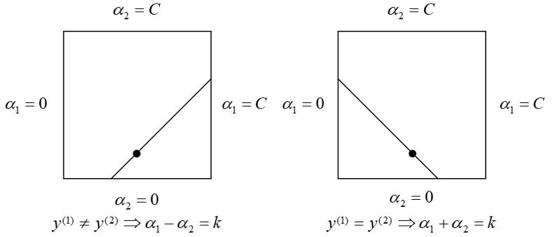
L ≤ α 2 n e w ≤ H L \leq \alpha_2^{new} \leq H L ≤ α 2 n e w ≤ H
where L and H are the two endpoints of the segment.
if y ( 1 ) ≠ y ( 2 ) y^{(1)} \neq y^{(2)} y ( 1 ) = y ( 2 )
L = max ( 0 , α 2 o l d − α 1 o l d ) , H = min ( C , C + α 2 o l d − α 1 o l d ) L=\max(0,\alpha_2^{old}-\alpha_1^{old}), H=\min(C,C+\alpha_2^{old}-\alpha_{1}^{old}) L = max ( 0 , α 2 o l d − α 1 o l d ) , H = min ( C , C + α 2 o l d − α 1 o l d )
if y ( 1 ) = y ( 2 ) y^{(1)} = y^{(2)} y ( 1 ) = y ( 2 )
L = max ( 0 , α 2 o l d + α 1 o l d − C ) , H = min ( C , α 2 o l d − α + 1 o l d ) L=\max(0,\alpha_2^{old}+\alpha_1^{old}-C), H=\min(C,\alpha_2^{old}-\alpha+{1}^{old}) L = max ( 0 , α 2 o l d + α 1 o l d − C ) , H = min ( C , α 2 o l d − α + 1 o l d )
Therefore,
α 2 new.clipped = { H , α 2 new > H α 2 new , L < α 2 new < H L , α 2 new ⩽ L \alpha_2^{\text {new.clipped }}= \begin{cases}H, & \alpha_2^{\text {new }}>H \\ \alpha_2^{\text {new }}, & L<\alpha_2^{\text {new }}<H \\ L, & \alpha_2^{\text {new }} \leqslant L\end{cases} α 2 new.clipped = ⎩ ⎪ ⎪ ⎨ ⎪ ⎪ ⎧ H , α 2 new , L , α 2 new > H L < α 2 new < H α 2 new ⩽ L
Further,with α 1 = ( ζ − α 2 y ( 2 ) ) , ζ = α 1 o l d y ( 1 ) + α 2 o l d y ( 2 ) \alpha_1=(\zeta-\alpha_{2}y^{(2)}),\zeta=\alpha_1^{old}y^{(1)}+\alpha_2^{old}y^{(2)} α 1 = ( ζ − α 2 y ( 2 ) ) , ζ = α 1 o l d y ( 1 ) + α 2 o l d y ( 2 )
α 1 n e w = ( α 1 o l d y ( 1 ) + α 2 o l d y ( 2 ) − α 2 n e w , c l i p p e d y ( 2 ) ) y ( 1 ) = α 1 o l d + y ( 1 ) y ( 2 ) ( α 2 o l d − α 2 n e w , c l i p p e d ) \begin{aligned}
\alpha_1^{new}&=(\alpha_1^{old}y^{(1)}+\alpha_2^{old}y^{(2)}-\alpha_2^{new,clipped}y^{(2)})y^{(1)}\\
&=\alpha_1^{old}+y^{(1)}y^{(2)}(\alpha_2^{old}-\alpha_2{new,clipped})
\end{aligned} α 1 n e w = ( α 1 o l d y ( 1 ) + α 2 o l d y ( 2 ) − α 2 n e w , c l i p p e d y ( 2 ) ) y ( 1 ) = α 1 o l d + y ( 1 ) y ( 2 ) ( α 2 o l d − α 2 n e w , c l i p p e d )
Solve the bias b
y ( 1 ) ( w ⊤ x ( 1 ) + b ) = y ( 1 ) g ( x ( 1 ) ) = y ( 1 ) ( ∑ i = 1 m α i y ( 1 ) K 1 i + b ) = 1 ∑ i = 1 m α i y ( i ) K 1 i + b = y ( 1 ) b 1 new = y ( 1 ) − ∑ i = 3 m α i y ( i ) K 1 i − α 1 new y ( 1 ) K 11 − α 2 new. clipped y ( 2 ) K 12 E 1 = ∑ i = 3 m α i y ( i ) K 1 i + α 1 old y ( 1 ) K 11 + α 2 old y ( 2 ) K 12 + b old − y ( 1 ) y^{(1)}\left(w^{\top} x^{(1)}+b\right)=y^{(1)} g\left(x^{(1)}\right)=y^{(1)}\left(\sum_{i=1}^m \alpha_i y^{(1)} K_{1 i}+b\right)=1
\\
\sum_{i=1}^m \alpha_i y^{(i)} K_{1 i}+b=y^{(1)}
\\
b_1^{\text {new }}=y^{(1)}-\sum_{i=3}^m \alpha_i y^{(i)} K_{1 i}-\alpha_1^{\text {new }} y^{(1)} K_{11}-\alpha_2^{\text {new. clipped }} y^{(2)} K_{12}
\\
E_1=\sum_{i=3}^m \alpha_i y^{(i)} K_{1 i}+\alpha_1^{\text {old }} y^{(1)} K_{11}+\alpha_2^{\text {old }} y^{(2)} K_{12}+b^{\text {old }}-y^{(1)} y ( 1 ) ( w ⊤ x ( 1 ) + b ) = y ( 1 ) g ( x ( 1 ) ) = y ( 1 ) ( ∑ i = 1 m α i y ( 1 ) K 1 i + b ) = 1 ∑ i = 1 m α i y ( i ) K 1 i + b = y ( 1 ) b 1 new = y ( 1 ) − ∑ i = 3 m α i y ( i ) K 1 i − α 1 new y ( 1 ) K 1 1 − α 2 new. clipped y ( 2 ) K 1 2 E 1 = ∑ i = 3 m α i y ( i ) K 1 i + α 1 old y ( 1 ) K 1 1 + α 2 old y ( 2 ) K 1 2 + b old − y ( 1 )
The first two terms in the above formula could be rewritten as:
y ( 1 ) − ∑ i = 3 m α i y ( i ) K 1 i = b old − E i + α 1 old y ( 1 ) K 11 + α 2 old y ( 2 ) K 12 y^{(1)}-\sum_{i=3}^m \alpha_i y^{(i)} K_{1 i}=b^{\text {old }}-E_i+\alpha_1^{\text {old }} y^{(1)} K_{11}+\alpha_2^{\text {old }} y^{(2)} K_{12} y ( 1 ) − ∑ i = 3 m α i y ( i ) K 1 i = b old − E i + α 1 old y ( 1 ) K 1 1 + α 2 old y ( 2 ) K 1 2
b 1 new = b old − E 1 − y ( 1 ) K 11 ( α 1 new − α 1 old ) − y ( 2 ) K 12 ( α 2 new. clipped − α 2 old ) b_1^{\text {new }}=b^{\text {old }}-E_1-y^{(1)} K_{11}\left(\alpha_1^{\text {new }}-\alpha_1^{\text {old }}\right)-y^{(2)} K_{12}\left(\alpha_2^{\text {new. clipped }}-\alpha_2^{\text {old }}\right) b 1 new = b old − E 1 − y ( 1 ) K 1 1 ( α 1 new − α 1 old ) − y ( 2 ) K 1 2 ( α 2 new. clipped − α 2 old )
When 0 ≤ α 2 new,clipped ≤ C 0 \le \alpha_2^{\text {new,clipped }} \le C 0 ≤ α 2 new,clipped ≤ C
b 2 new = b old − E 2 − y ( 1 ) K 12 ( α 1 new − α 1 old ) − y ( 2 ) K 22 ( α 2 new clipped − α 2 old ) b_2^{\text {new }}=b^{\text {old }}-E_2-y^{(1)} K_{12}\left(\alpha_1^{\text {new }}-\alpha_1^{\text {old }}\right)-y^{(2)} K_{22}\left(\alpha_2^{\text {new clipped }}-\alpha_2^{\text {old }}\right) b 2 new = b old − E 2 − y ( 1 ) K 1 2 ( α 1 new − α 1 old ) − y ( 2 ) K 2 2 ( α 2 new clipped − α 2 old )
Therefore,
b new = { b 1 new , 0 < α 1 new < C b 2 new , 0 ≤ α 2 new, clipped ≤ C ( b 1 n e w + b 2 n e w ) 2 O t h e r b^{\text {new }}= \begin{cases}b_1^{\text {new }}, & 0<\alpha_1^{\text {new }}<C \\
b_2^{\text {new }}, & 0 \le \alpha_2^{\text {new, clipped }} \le C \\
\frac{(b_{1}^{new}+b_{2}^{new})}{2} & Other \end{cases} b new = ⎩ ⎪ ⎪ ⎨ ⎪ ⎪ ⎧ b 1 new , b 2 new , 2 ( b 1 n e w + b 2 n e w ) 0 < α 1 new < C 0 ≤ α 2 new, clipped ≤ C O t h e r
Code 1 2 3 4 5 6 7 8 9 10 11 12 13 14 15 16 17 18 19 20 21 22 23 24 25 26 27 28 29 30 31 32 33 34 35 36 37 38 39 40 41 42 43 44 45 46 47 48 49 50 51 52 53 54 55 56 57 58 59 60 61 62 63 64 65 66 67 68 69 70 71 72 73 74 75 76 77 78 79 80 81 82 83 84 85 86 87 88 89 90 91 92 93 94 95 96 97 98 99 100 101 102 103 104 105 106 107 108 109 110 111 112 113 114 115 116 117 118 119 import numpy as npdef compute_w (data_x, data_y, alphas ): p1 = data_y.reshape(-1 , 1 ) * data_x p2 = alphas.reshape(-1 , 1 ) * p1 return np.sum (p2, axis=0 ) def kernel (x1, x2 ): return np.dot(x1, x2) def f_x (data_x, data_y, alphas, x, b ): k = kernel(data_x, x) r = alphas * data_y * k return np.sum (r) + b def compute_L_H (C, alpha_i, alpha_j, y_i, y_j ): L = np.max ((0. , alpha_j - alpha_i)) H = np.min ((C, C + alpha_j - alpha_i)) if y_i == y_j: L = np.max ((0. , alpha_i + alpha_j - C)) H = np.min ((C, alpha_i + alpha_j)) return L, H def compute_eta (x_i, x_j ): return 2 * kernel(x_i, x_j) - kernel(x_i, x_i) - kernel(x_j, x_j) def compute_E_k (f_x_k, y_k ): return f_x_k - y_k def clip_alpha_j (alpha_j, H, L ): if alpha_j > H: return H if alpha_j < L: return L return alpha_j def compute_alpha_j (alpha_j, E_i, E_j, y_j, eta ): return alpha_j - (y_j * (E_i - E_j) / eta) def compute_alpha_i (alpha_i, y_i, y_j, alpha_j, alpha_old_j ): return alpha_i + y_i * y_j * (alpha_old_j - alpha_j) def compute_b1 (b, E_i, y_i, alpha_i, alpha_old_i, x_i, y_j, alpha_j, alpha_j_old, x_j ): p1 = b - E_i - y_i * (alpha_i - alpha_old_i) * kernel(x_i, x_i) p2 = y_j * (alpha_j - alpha_j_old) * kernel(x_i, x_j) return p1 - p2 def compute_b2 (b, E_j, y_i, alpha_i, alpha_old_i, x_i, x_j, y_j, alpha_j, alpha_j_old ): p1 = b - E_j - y_i * (alpha_i - alpha_old_i) * kernel(x_i, x_j) p2 = y_j * (alpha_j - alpha_j_old) * kernel(x_j, x_j) return p1 - p2 def clip_b (alpha_i, alpha_j, b1, b2, C ): if alpha_i > 0 and alpha_i < C: return b1 if alpha_j > 0 and alpha_j < C: return b2 return (b1 + b2) / 2 def select_j (i, m ): j = np.random.randint(m) while i == j: j = np.random.randint(m) return j def smo (C, tol, max_passes, data_x, data_y ): m, n = data_x.shape b, passes = 0. , 0 alphas = np.zeros(shape=(m)) alphas_old = np.zeros(shape=(m)) while passes < max_passes: num_changed_alphas = 0 for i in range (m): x_i, y_i, alpha_i = data_x[i], data_y[i], alphas[i] f_x_i = f_x(data_x, data_y, alphas, x_i, b) E_i = compute_E_k(f_x_i, y_i) if ((y_i * E_i < -tol and alpha_i < C) or (y_i * E_i > tol and alpha_i > 0. )): j = select_j(i, m) x_j, y_j, alpha_j = data_x[j], data_y[j], alphas[j] f_x_j = f_x(data_x, data_y, alphas, x_j, b) E_j = compute_E_k(f_x_j, y_j) alphas_old[i], alphas_old[j] = alpha_i, alpha_j L, H = compute_L_H(C, alpha_i, alpha_j, y_i, y_j) if L == H: continue eta = compute_eta(x_i, x_j) if eta >= 0 : continue alpha_j = compute_alpha_j(alpha_j, E_i, E_j, y_j, eta) alpha_j = clip_alpha_j(alpha_j, H, L) alphas[j] = alpha_j if np.abs (alpha_j - alphas_old[j]) < 10e-5 : continue alpha_i = compute_alpha_i(alpha_i, y_i, y_j, alpha_j, alphas_old[j]) b1 = compute_b1(b, E_i, y_i, alpha_i, alphas_old[i], x_i, y_i, alpha_j, alphas_old[j], x_j) b2 = compute_b2(b, E_j, y_i, alpha_i, alphas_old[i], x_i, x_j, y_j, alpha_j, alphas_old[j]) b = clip_b(alpha_i, alpha_j, b1, b2, C) num_changed_alphas += 1 alphas[i] = alpha_i if num_changed_alphas == 0 : passes += 1 else : passes = 0 return alphas, b
Reference Andrew Ng, Machine Learning, Stanford University